Introducing alarmdata

The first stable version of our package alarmdata is now on CRAN, introducing a data-focused package for using the outputs of ALARM Project research.

alarmdata is the newest component of the redistverse, a family of packages which provide tools for redistricting analyses in R. As of the past weekend, it is now on CRAN. You can install the following with:

install.packages('alarmdata')

Downloading data

alarmdata provides several functions for loading in data from ALARM Project projects. Most useful are alarm_50state_map() and alarm_50state_plans() which respectively load in the maps and plans from our 50-states project. The map object contains Census and election for each state precinct. The plans object contains alternative simulated plans.

To download and use these data, you can use the following code:

library(alarmdata)
library(redist)

map_wa <- alarm_50state_map('WA')
plans_wa <- alarm_50state_plans('WA')

Using redist_map objects

redist provides an extension to tibbles, called a redist_map. This builds on the sf tibble class and adds an adjacency column to the data. The adjacency column is modeled on each state’s particular definition of contiguity. For example, in Washington, contiguity across water is not considered unless there is a ferry route there. This makes it easy to plug into redist’s sampling functions, like redist_smc or redist_mergesplit.

Even for those not running simulation analyses, the redist_map can still be useful, as it is just an extension of the sf class. Each object contains the enacted 2010 and 2020 congressional plans. They also contain census variables such as total population (pop), voting age population vap, and the major racial categories (e.g. pop_white or vap_black).

redist_maps also include election data, which are retabulations of VEST’s election data to census shapes. Election data follows a pattern of office_year_party_candidate, like pre_16_dem_cli for Clinton’s 2016 presidential votes. Year averages take the form adv_year for Democratic votes and arv_year for Republican votes (e.g. arv_20 or adv_20). Finally, the redist_map also includes a ndv and nrv column, which are the average of Democratic and Republican votes in each shape, respectively.

Given all this, it interfaces nicely with ggplot2 for making maps. Here, we can also load the ggredist package for some nice election mapping functions and colors. To make a precinct map, we could run the following:

library(ggplot2)
library(ggredist)
map_wa |> 
    ggplot() +
    geom_sf(aes(fill = ndv / (nrv + ndv))) +
    scale_fill_party_c() +
    theme_map()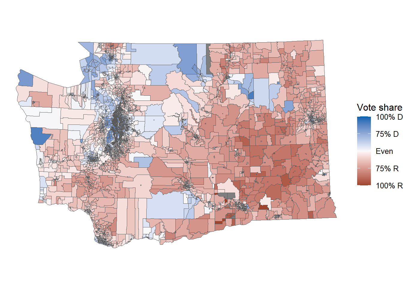

To make a 2020 district map, we can swap out the geom call:

map_wa |> 
    ggplot() +
    geom_district(aes(group = cd_2020, fill = ndv, denom = nrv + ndv)) +
    scale_fill_party_c() +
    theme_map()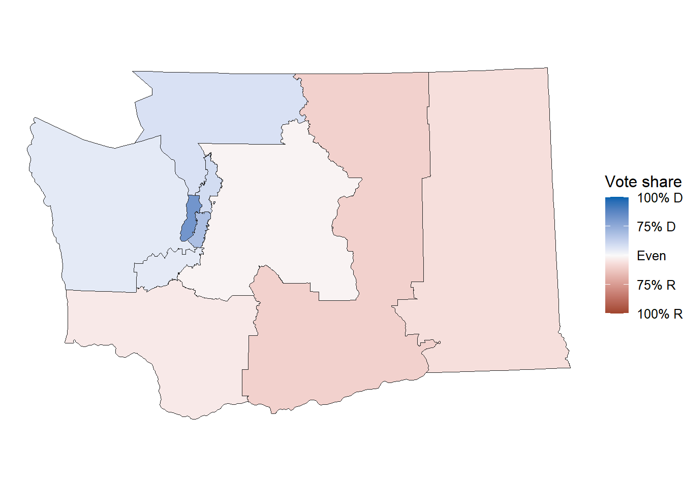

Using redist_plans with your own data

Once you’ve downloaded some plans, we’ve made it easy for you to add your own data to the redist framework. To demo this, we can look at the NY plans passed last week (February 2024).

First, we can load in the map and plans for New York:

map_ny <- alarm_50state_map('NY')
plans_ny <- alarm_50state_plans('NY')

Next, we can read in the block assignment data for the commission plan and the legislature plan. For convenience of the example, we can grab this data from a GitHub repo.

# commission link
comm_link <- 'https://raw.githubusercontent.com/christopherkenny/ny-baf/main/data/A09310.csv'

# download the legislature xlsx file
leg_link <- 'https://github.com/christopherkenny/ny-baf/raw/main/data-raw/congressional_plan_equivalency.xlsx'
temp_leg <- tempfile(fileext = '.xlsx')
curl::curl_download(leg_link, temp_leg)

# read in the data
baf_commission <- readr::read_csv(comm_link, col_types = 'ci') |> 
  dplyr::rename(A09310 = district)
baf_legislature <- readxl::read_excel(temp_leg, col_types = c('text', 'text')) |> 
  dplyr::rename(
    GEOID = Block,
    commission2024 = `DistrictID:1`
  ) |> 
  dplyr::mutate(commission2024 = as.integer(commission2024))

Finally, alarmdata provides a function alarmdata::alarm_add_plan() to add the new reference plans to the underlying redist_plans object.

plans_ny <- plans_ny |>
  alarm_add_plan(ref_plan = baf_commission, map = map_ny, name = 'A09310') |>
  alarm_add_plan(ref_plan = baf_legislature, map = map_ny, name = 'commission2024')

This gives a full redist_plans object with the new plans added in. We can do anything we want with this. For example, stealing a bit of code from our 50-states website, we can look at the Democratic vote shares across districts:

First, we can define some helper functions for the plot:

lbl_party <- function(x) {
  dplyr::if_else(x == 0.5, "Even",
    paste0(dplyr::if_else(x < 0.5, "R+", "D+"), scales::number(200 * abs(x - 0.5), 1))
  )
}

r_geom <- function(...) {
  ggplot2::geom_point(
    ggplot2::aes(x = as.integer(.data$.distr_no),
                 y = e_dvs,
                 color = .data$draw, 
                 shape = .data$draw),
    ...
  )
}

Then, we can make a simple plot of Democratic vote share by district:

library(ggplot2)
library(ggredist)
redist.plot.distr_qtys(plans_ny, e_dvs,
                       color_thresh = 0.5,
                       size = 0.04 - sqrt(8) / 250, alpha = 0.4,
                       ref_geom = r_geom
) +
    geom_hline(yintercept = 0.5, color = '#00000055', size = 0.5) +
    scale_y_continuous('Two-party vote margin', labels = lbl_party) +
    labs(x = 'Simulated districts, ordered by Democratic vote margin') +
    annotate('text',
             x = 3.5, y = sort(plans_ny$e_dvs[1:26])[3],
             label = 'Commission 2024', hjust = -0.05, size = 3.5,
             color = '#52796F'
    ) +
    annotate('text',
             x = 1.5, y = min(plans_ny$e_dvs[27:52]),
             label = 'A09310', hjust = 0.05, size = 3.5,
             color = '#A09310'
    ) +
    annotate('text',
             x = 3.5, y = sort(plans_ny$e_dvs[53:78])[3],
             label = 'Cervas', hjust = -0.05, size = 3.5,
             color = 'black'
    ) + 

    scale_color_manual(values = c('#52796F', '#A09310', 'black', ggredist$partisan[2], ggredist$partisan[14]),
                       labels = c('pt', 'Rep.', 'Dem.'), guide = 'none') +
    scale_shape_manual(values = c(16, 17, 18), guide = 'none') +
    theme_bw()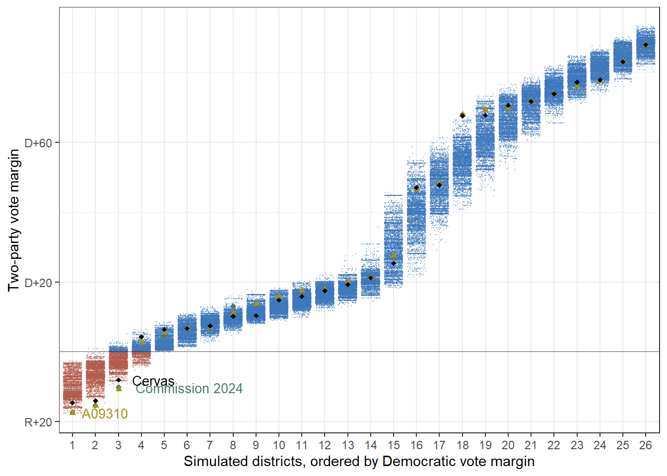

Cache data across projects

By default, all downloads are directed to a temporary directory. Each time you reload R, you need to re-download the data. To avoid this, you can set the alarm.use_cache option to a directory where you want to store the data.

options(alarm.use_cache = TRUE)

This can be set on a by-session basis, but we recommend setting it in your .Rprofile so that it is set every time you start R. To open this file, use the following command:

usethis::edit_r_profile()