The redist package provides algorithms and tools for
scalable and replicable redistricting analyses. This vignette introduces
the package by way of an analysis of redistricting in the state of Iowa,
which can broken down into four distinct steps:
- Compiling, cleaning, and preparing the data
- Defining the redistricting problem
- Simulating redistricting plans
- Analyzing the simulated plans
First, however, a brief overview of the package itself.
The redist package
To install redist, follow the instructions in the README.
For more information on package components, check out the full documentation.
Algorithms
The package contains a variety of redistricting simulation and enumeration algorithms. Generally you will use one of the following three algorithms:
-
redist_smc(), the recommended algorithm for most purposes.1 -
redist_mergesplit(), a MCMC version of the SMC proposal.2 -
redist_flip(), another MCMC algorithm which uses more local proposals.3
The other algorithms are
-
redist.enumpart()for efficient enumeration of small maps.4 -
redist_shortburst()for optimizing a plan according to a user-provided criterion.5 -
redist.rsg()andredist.crsg(), which do not sample from a known target distribution.6
Compiling, cleaning, and preparing the data
The most time-consuming part of a redistricting analysis, like most data analyses, is collecting and cleaning the necessary data. For redistricting, this data includes geographic shapefiles for precincts and existing legislative district plans, precinct- or block-level demographic information from the Census, and precinct-level political data. These data generally come from different sources, and may not fully overlap with each other, further complicating the problem.
redist is not focused on this data collection process.
The geomander
package contains many helpful functions for compiling these data, and
fixing problems in geographic data.
The ALARM project provides pre-cleaned redistricting data files consisting of VEST election data joined 2020 Census data at the precinct level. Other sources for precinct-level geographic and political information include the MIT Election Lab, the Census, the Redistricting Data Hub, the Voting and Election Science Team, the Harvard Election Data Archive, the Metric Geometry and Gerrymandering Group, and some state websites.
Iowa
For this analysis of Iowa, we’ll use the data included in the
package, which was compiled from the Census and the Harvard Election
Data Archive. It contains, for each county, the total population and
voting-age population by race, as well as the number of votes for
President in 2008. The geometry column contains the
geographic shapefile
information.
data(iowa)
print(iowa)
#> Simple feature collection with 99 features and 15 fields
#> Geometry type: MULTIPOLYGON
#> Dimension:     XY
#> Bounding box:  xmin: 4081849 ymin: 2879102 xmax: 5834228 ymax: 4024957
#> Projected CRS: NAD83(HARN) / Iowa North (ftUS)
#> First 10 features:
#>     fips       name cd_2010    pop  white black hisp    vap  wvap bvap hvap
#> 1  19001      Adair       3   7682   7507    11  101   5957  5860    5   53
#> 2  19003      Adams       3   4029   3922     8   37   3180  3109    6   22
#> 3  19005  Allamakee       1  14330  13325   109  757  11020 10430   82  425
#> 4  19007  Appanoose       2  12887  12470    55  181   9993  9745   40   99
#> 5  19009    Audubon       4   6119   6007     9   37   4780  4714    5   27
#> 6  19011     Benton       1  26076  25387    93  275  19430 19068   49  155
#> 7  19013 Black Hawk       1 131090 109968 11493 4907 102594 89541 7677 2865
#> 8  19015      Boone       4  26306  25194   202  505  20027 19448  103  260
#> 9  19017     Bremer       1  24276  23459   186  239  18763 18242  155  137
#> 10 19019   Buchanan       1  20958  20344    59  243  15282 14979   32  128
#>    tot_08 dem_08 rep_08    region                       geometry
#> 1    4053   1924   2060     South MULTIPOLYGON (((4592338 328...
#> 2    2206   1118   1046     South MULTIPOLYGON (((4528041 315...
#> 3    7059   3971   2965 Northeast MULTIPOLYGON (((5422507 401...
#> 4    6176   2970   3086     South MULTIPOLYGON (((5032545 306...
#> 5    3435   1739   1634 Northwest MULTIPOLYGON (((4487363 341...
#> 6   13712   7058   6447 Southeast MULTIPOLYGON (((5246216 357...
#> 7   64775  39184  24662 Northeast MULTIPOLYGON (((5175640 369...
#> 8   13929   7356   6293   Central MULTIPOLYGON (((4741174 354...
#> 9   12871   6940   5741 Northeast MULTIPOLYGON (((5174636 379...
#> 10  10338   6050   4139 Northeast MULTIPOLYGON (((5302846 370...
Defining the redistricting problem
A redistricting problem is defined by the map of the precincts, the number of contiguous districts to divide the precincts into, the level of population parity to enforce, and any other necessary constraints that must be imposed.
Determining the relevant constraints
In Iowa, congressional districts are constructed not out of precincts but out of the state’s 99 counties, and in the 2010 redistricting cycle, Iowa was apportioned four congressional districts, down one from the 2000 cycle. Chapter 42 of the Iowa Code provides guidance on the other constraints imposed on the redistricting process (our emphasis added):
42.4 Redistricting standards.
…
1.b. Congressional districts shall each have a population as nearly equal as practicable to the ideal district population, derived as prescribed in paragraph “a” of this subsection. No congressional district shall have a population which varies by more than one percent from the applicable ideal district population, except as necessary to comply with Article III, section 37 of the Constitution of the State of Iowa.
…
3. Districts shall be composed of convenient contiguous territory. Areas which meet only at the points of adjoining corners are not contiguous.
4. Districts shall be reasonably compact in form, to the extent consistent with the standards established by subsections 1, 2, and 3. In general, reasonably compact districts are those which are square, rectangular, or hexagonal in shape, and not irregularly shaped, to the extent permitted by natural or political boundaries….
5. No district shall be drawn for the purpose of favoring a political party, incumbent legislator or member of Congress, or other person or group, or for the purpose of augmenting or diluting the voting strength of a language or racial minority group. In establishing districts, no use shall be made of any of the following data:
- Addresses of incumbent legislators or members of Congress.
- Political affiliations of registered voters.
- Previous election results.
- Demographic information, other than population head counts, except as required by the Constitution and the laws of the United States.
The section goes on to provide two specific measures of compactness that should be used to compare districts, one of which is the total perimeter of all districts. If the total perimeter is small, then the districts relatively compact.
Contiguity of districts and no reliance on partisan or demographic
data are built-in to redist. We’ll look at how to specify
the desired population deviation (no more than 1% by law) in the next
section, and discuss compactness in the simulation
section.
Setting up the problem in redist
In redist, a basic redistricting problem is defined by
an object of type redist_map, which can be constructed
using the eponymous function. The user must provide a vector of
population counts (defaults to the pop column, if one
exists) and the desired population parity, and the number of districts.
The latter can be inferred if a reference redistricting plan exists. For
Iowa, we’ll use the adopted 2010 plan as a reference.
iowa_map = redist_map(iowa, existing_plan=cd_2010, pop_tol=0.01, total_pop = pop)
print(iowa_map)
#> A <redist_map> with 99 units and 17 fields
#> To be partitioned into 4 districts with population between 761,588.8 - 1.0% and 761,588.8 + 1.0%
#> With geometry:
#>     bbox:           xmin: 4081849 ymin: 2879102 xmax: 5834228 ymax: 4024957
#>     projected CRS:  NAD83(HARN) / Iowa North (ftUS)
#> # A tibble: 99 × 17
#>    fips  name  cd_2010    pop  white black  hisp    vap  wvap  bvap  hvap tot_08
#>  * <chr> <chr>   <int>  <dbl>  <dbl> <dbl> <dbl>  <dbl> <dbl> <dbl> <dbl>  <dbl>
#>  1 19001 Adair       3   7682   7507    11   101   5957  5860     5    53   4053
#>  2 19003 Adams       3   4029   3922     8    37   3180  3109     6    22   2206
#>  3 19005 Alla…       1  14330  13325   109   757  11020 10430    82   425   7059
#>  4 19007 Appa…       2  12887  12470    55   181   9993  9745    40    99   6176
#>  5 19009 Audu…       4   6119   6007     9    37   4780  4714     5    27   3435
#>  6 19011 Bent…       1  26076  25387    93   275  19430 19068    49   155  13712
#>  7 19013 Blac…       1 131090 109968 11493  4907 102594 89541  7677  2865  64775
#>  8 19015 Boone       4  26306  25194   202   505  20027 19448   103   260  13929
#>  9 19017 Brem…       1  24276  23459   186   239  18763 18242   155   137  12871
#> 10 19019 Buch…       1  20958  20344    59   243  15282 14979    32   128  10338
#> # ℹ 89 more rows
#> # ℹ 5 more variables: dem_08 <dbl>, rep_08 <dbl>, region <chr>,
#> #   geometry <MULTIPOLYGON [US_survey_foot]>, adj <list>
This looks much the same as iowa itself, but metadata
has been added, and there’s a new column, adj.
Adjacency-based redistricting
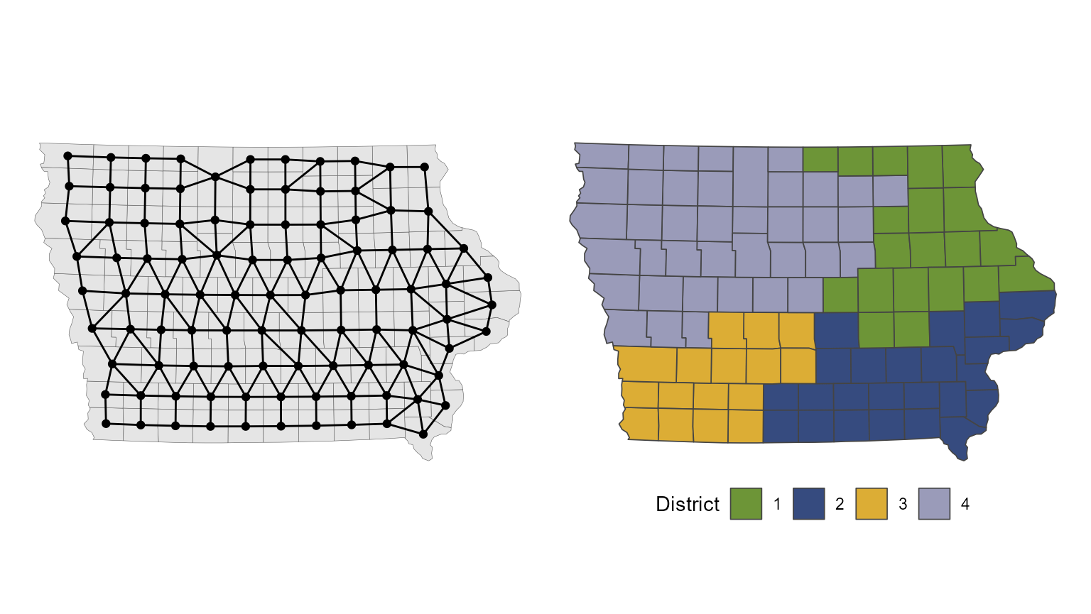
All redistricting algorithms operate on an adjacency graph, which is constructed from the actual precinct or county geography. In the adjacency graph, every precinct or county is a node, and two nodes are connected by an edge if the corresponding precincts are geographically adjacent.7 Creating a contiguous set of districts as part of a redistricting plan then corresponds to creating a partition of the adjacency graph.
The redist_map() function automatically computes the
adjacency graph from the provided shapefile (though one can be provided
directly as well), and stores it in the adj column as an
adjacency list, which is, for each precinct, a list of
neighboring precincts. As part of this process, the adjacency graph is
checked for global contiguity (no islands), which is necessary for the
redistricting algorithms to function properly.
We can visualize the adjacency graph by plotting the
redist_map object.
Pre-processing
Often, we want to only analyze a portion of a map, or hold some districts fixed while others are re-simulated. We may also want to implement a status-quo-type constraint that encourages simulated districts to be close to a reference plan. This can be accomplished by freezing the “cores” of each district.
All of these operations fall under the umbrella of map
pre-processing, and redist is well-equipped to handle them.
You can use familiar dplyr verbs like filter()
and summarize(), along with new redist
operations like freeze(), make_cores(), and
merge_by(), to operate on redist_map objects.
The package will make the appropriate modifications to the geometry and
adjacency graph in the background.
The map pre-processing vignette contains more information and examples about these operations.
Exploring the geography
To get a feel for the demographic and political geography of the
state, we’ll make some plots from the iowa_map object. We
see that the state is mostly rural and white, with Polk county (Des
Moines) the largest and densest. Politically, most counties are
relatively balanced between Democrats and Republicans (at least in the
’08 election), though there is a rough east-west gradient.
areas = as.numeric(units::set_units(sf::st_area(iowa_map$geometry), mi^2))
plot(iowa_map, fill = pop / areas) +
    scale_fill_viridis_c(name="Population density (people / sq. mi)",
                         trans="sqrt")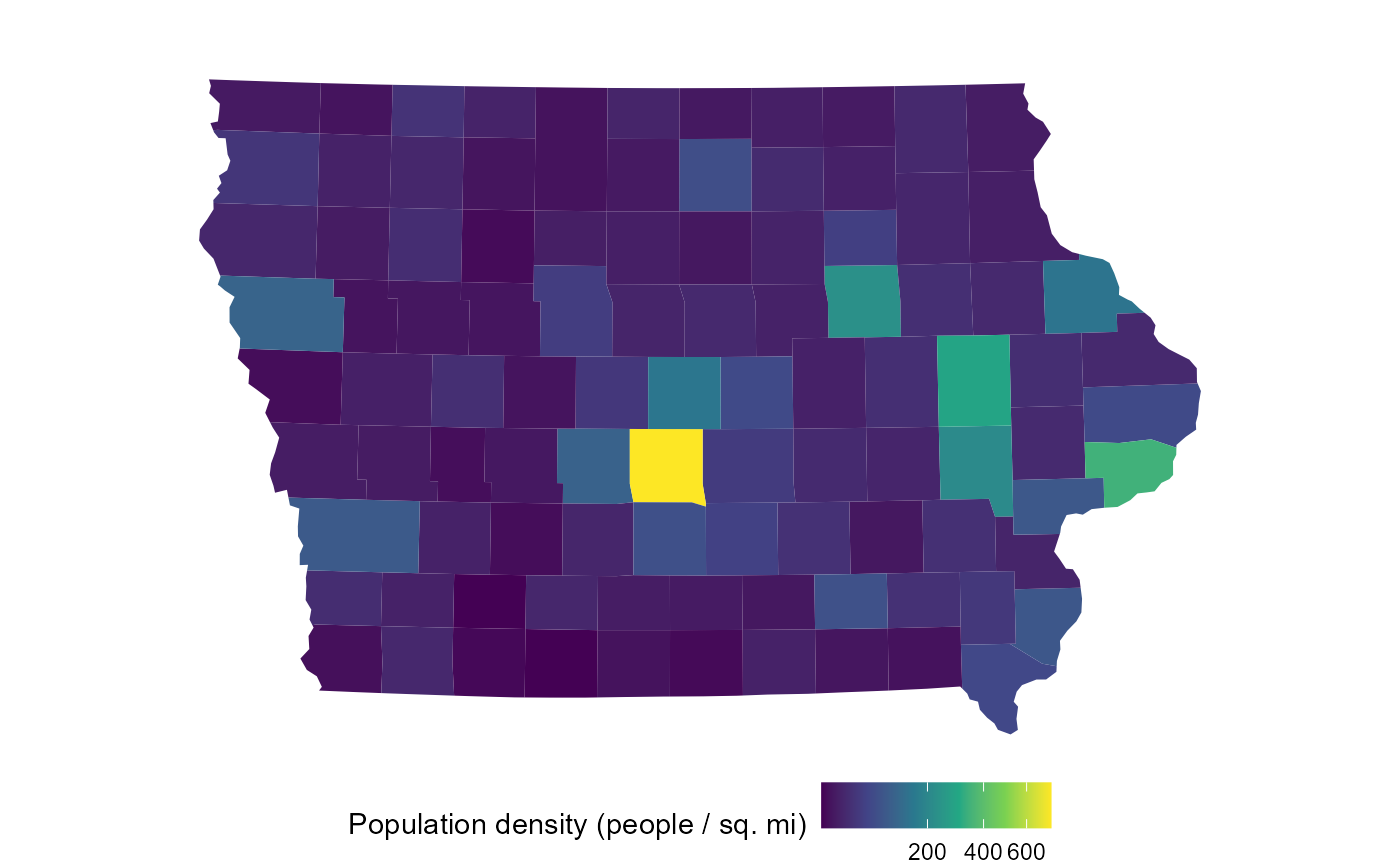
plot(iowa_map, fill = dem_08 / tot_08) +
    scale_fill_gradient2(name="Pct. Democratic '08",  midpoint=0.5)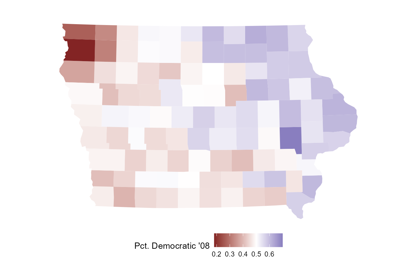
plot(iowa_map, fill = wvap / vap, by_distr = TRUE)
Simulating redistricting plans
The crux of a redistricting analysis is actually simulating new
redistricting plans. As discussed above, redist provides
several algorithms for performing this simulation, and each has its own
advantages and incorporates a different set of constraints. Here, we’ll
demonstrate use of the redist_smc() algorithm, a Sequential
Monte Carlo (SMC)-based procedure which is the recommended choice for
most redistricting analyses.
SMC creates plans directly, by drawing district boundaries one at a time, as illustrated below.

Because of the way districts are drawn in SMC, the generated
districts are relatively compact by default. This can be further
controlled by the compactness parameter (although
compactness=1 is particularly computationally
convenient).
To simulate, we call redist_smc() on our
redist_map object. We provide the runs=2
parameter, which will run the SMC algorithm twice, in parallel. This
doubles the total number of sampled plans, but more importantly, it
provides extremely valuable diagnostic information about whether the
algorithm is sampling properly.
iowa_plans = redist_smc(iowa_map, 500, compactness=1, runs=2)The output from the algorithm is a redist_plans object,
which stores a matrix of district assignments for each precinct and
simulated plans, and a table of summary statistics for each district and
simulated plan. The existing 2010 plan has also been automatically added
as a reference plan. Additional reference or comparison plans may be
added using add_reference().
print(iowa_plans)
#> A <redist_plans> containing 1,000 sampled plans and 1 reference plan
#> Plans have 4 districts from a 99-unit map, and were drawn using Sequential
#> Monte Carlo.
#> With plans resampled from weights
#> Plans matrix: int [1:99, 1:1001] 1 1 2 3 4 2 2 4 2 2 ...
#> # A tibble: 4,004 × 4
#>    draw    district total_pop chain
#>    <fct>      <int>     <dbl> <int>
#>  1 cd_2010        1    761612    NA
#>  2 cd_2010        2    761548    NA
#>  3 cd_2010        3    761624    NA
#>  4 cd_2010        4    761571    NA
#>  5 1              1    759274     1
#>  6 1              2    763216     1
#>  7 1              3    755788     1
#>  8 1              4    768077     1
#>  9 2              1    759558     1
#> 10 2              2    761089     1
#> # ℹ 3,994 more rows
We can explore specific simulated plans with
redist.plot.plans().
redist.plot.plans(iowa_plans, draws=1:6, shp=iowa_map)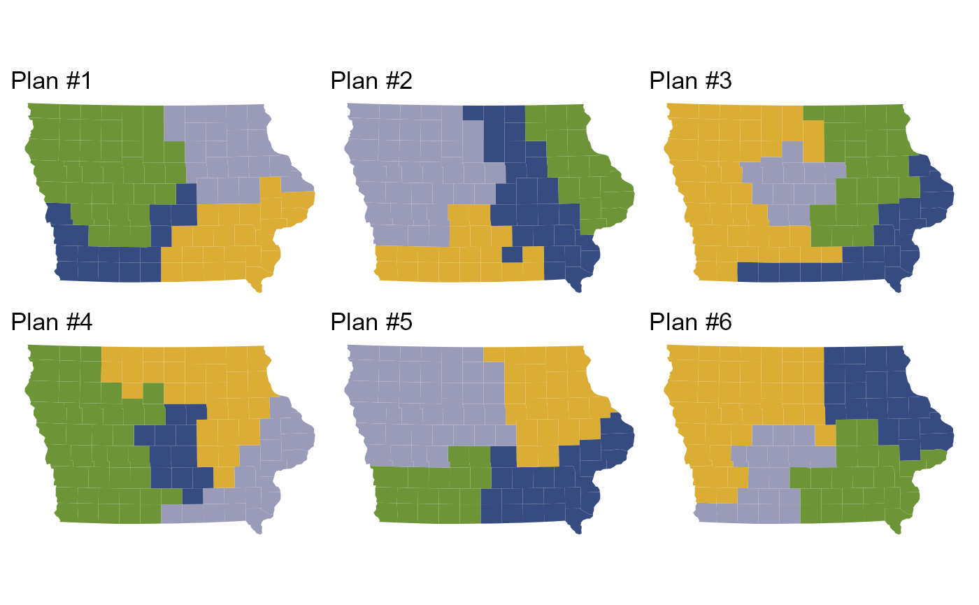
Analyzing the simulated plans
A redist_plans object, the output of a sampling
algorithm, links a matrix of precinct assignments to a table of district
statistics, and this linkage makes analyzing the output a breeze.
Sometimes it may be useful to renumber the simulated districts (which
have random numbers in general) to match the reference plan as closely
as possible. This adds a pop_overlap column which measures
how much of the population is in the same district in both a given plan
and the reference plan.
iowa_plans = match_numbers(iowa_plans, iowa_map$cd_2010)
print(iowa_plans)
#> A <redist_plans> containing 1,000 sampled plans and 1 reference plan
#> Plans have 4 districts from a 99-unit map, and were drawn using Sequential
#> Monte Carlo.
#> With plans resampled from weights
#> Plans matrix: int [1:99, 1:1001] 3 3 1 2 4 1 1 4 1 1 ...
#> # A tibble: 4,004 × 5
#>    draw    district total_pop chain pop_overlap
#>    <fct>   <ord>        <dbl> <int>       <dbl>
#>  1 cd_2010 1           761548    NA       1
#>  2 cd_2010 2           761624    NA       1
#>  3 cd_2010 3           761612    NA       1
#>  4 cd_2010 4           761571    NA       1
#>  5 1       1           768077     1       0.738
#>  6 1       2           763216     1       0.738
#>  7 1       3           755788     1       0.738
#>  8 1       4           759274     1       0.738
#>  9 2       1           766367     1       0.639
#> 10 2       2           761089     1       0.639
#> # ℹ 3,994 more rows
Then we can add summary statistics by district, using
redist’s analysis functions. Here, we’ll compute the
population deviation, the perimeter-based compactness measure related to
the Iowa Code’s redistricting requirements, and the fraction of minority
voters and two-party Democratic vote share by district.
county_perims = prep_perims(iowa_map, iowa_map$adj)

iowa_plans = iowa_plans %>%
    mutate(pop_dev = abs(total_pop / get_target(iowa_map) - 1),
           comp = comp_polsby(pl(), iowa_map, perim_df=county_perims),
           pct_min = group_frac(iowa_map, vap - wvap, vap),
           pct_dem = group_frac(iowa_map, dem_08, dem_08 + rep_08))
print(iowa_plans)
#> With plans resampled from weights
#> Plans matrix: int [1:99, 1:1001] 3 3 1 2 4 1 1 4 1 1 ...
#> # A tibble: 4,004 × 9
#>    draw    district total_pop chain pop_overlap   pop_dev  comp pct_min pct_dem
#>    <fct>   <ord>        <dbl> <int>       <dbl>     <dbl> <dbl>   <dbl>   <dbl>
#>  1 cd_2010 1           761548    NA       1     0.0000535 0.302  0.0737   0.592
#>  2 cd_2010 2           761624    NA       1     0.0000463 0.360  0.0968   0.579
#>  3 cd_2010 3           761612    NA       1     0.0000305 0.529  0.114    0.531
#>  4 cd_2010 4           761571    NA       1     0.0000233 0.522  0.0788   0.491
#>  5 1       1           768077     1       0.738 0.00852   0.503  0.0646   0.593
#>  6 1       2           763216     1       0.738 0.00214   0.415  0.0955   0.577
#>  7 1       3           755788     1       0.738 0.00762   0.515  0.129    0.563
#>  8 1       4           759274     1       0.738 0.00304   0.428  0.0741   0.456
#>  9 2       1           766367     1       0.639 0.00627   0.402  0.0738   0.577
#> 10 2       2           761089     1       0.639 0.000656  0.246  0.103    0.609
#> # ℹ 3,994 more rows
Once summary statistics of interest have been calculated, it’s very
important to check the algorithm’s diagnostics. As with any complex
sampling algorithm, things can go wrong. Diagnostics, while not
flawless, can help catch problems and stop you from making conclusions
that are actually the fault of a broken sampling process. The
summary() function is redist’s one-stop-shop
for algorithm diagnostics.
summary(iowa_plans)
#> SMC: 1,000 sampled plans of 4 districts on 99 units
#> `adapt_k_thresh`=0.99 • `seq_alpha`=0.5
#> `pop_temper`=0
#> Plan diversity 80% range: 0.47 to 0.80
#>
#> R-hat values for summary statistics:
#> pop_overlap     pop_dev        comp     pct_min     pct_dem
#>       1.004       1.000       0.999       1.000       0.999
#> Sampling diagnostics for SMC run 1 of 2 (500 samples)
#>          Eff. samples (%) Acc. rate Log wgt. sd  Max. unique Est. k
#> Split 1       492 (98.4%)      5.5%        0.25   313 ( 99%)      5
#> Split 2       484 (96.9%)      6.6%        0.34   297 ( 94%)      4
#> Split 3       477 (95.5%)      3.0%        0.41   279 ( 88%)      3
#> Resample      410 (82.0%)       NA%        0.41   406 (128%)     NA
#> Sampling diagnostics for SMC run 2 of 2 (500 samples)
#>          Eff. samples (%) Acc. rate Log wgt. sd  Max. unique Est. k
#> Split 1       492 (98.4%)      9.9%        0.26   313 ( 99%)      3
#> Split 2       480 (96.1%)      9.7%        0.38   324 (103%)      3
#> Split 3       479 (95.7%)      4.7%        0.42   275 ( 87%)      2
#> Resample      422 (84.4%)       NA%        0.42   417 (132%)     NA
#> •  Watch out for low effective samples, very low acceptance rates (less than
#> 1%), large std. devs. of the log weights (more than 3 or so), and low numbers
#> of unique plans. R-hat values for summary statistics should be between 1 and
#> 1.05.
There’s a lot of diagnostic output there, which you should read more
about with ?summary.redist_plans. If anything is obviously
wrong, the function will alert you and provide instructions on how to
try to fix it. But these warnings aren’t flawless, and it’s important to
check the numbers yourself.
If you’ve used 2 or more runs, as we have,
summary() will calculate R-hat values. These should be as
close to 1 as possible, and generally less than 1.05. If they are bigger
than that, it means that multiple independent runs of the algorithm gave
different results. More samples (higher nsims) are usually
called for. The other number to keep an eye on is the plan diversity
(top of the output), whose 80% range should generally cover the range
from 0.5–0.8.
Since our diagnostics look good, we can return to our analysis. It’s
quick to turn district-level statistics from a redist_plans
object into plan-level summary statistics.
plan_sum = group_by(iowa_plans, draw) %>%
    summarize(max_dev = max(pop_dev),
              avg_comp = mean(comp),
              max_pct_min = max(pct_min),
              dem_distr = sum(pct_dem > 0.5))
print(plan_sum)
#> A <redist_plans> containing 1,000 sampled plans and 1 reference plan
#> Plans have 4 districts from a 99-unit map, and were drawn using Sequential
#> Monte Carlo.
#> With plans resampled from weights
#> Plans matrix: int [1:99, 1:1001] 3 3 1 2 4 1 1 4 1 1 ...
#> # A tibble: 1,001 × 5
#>    draw      max_dev avg_comp max_pct_min dem_distr
#>    <fct>       <dbl>    <dbl>       <dbl>     <int>
#>  1 cd_2010 0.0000535    0.428       0.114         3
#>  2 1       0.00852      0.465       0.129         3
#>  3 2       0.00627      0.379       0.110         3
#>  4 3       0.00290      0.403       0.127         3
#>  5 4       0.00888      0.333       0.122         4
#>  6 5       0.00660      0.371       0.109         3
#>  7 6       0.00697      0.334       0.118         3
#>  8 7       0.00686      0.414       0.111         3
#>  9 8       0.00778      0.445       0.109         3
#> 10 9       0.00361      0.382       0.123         3
#> # ℹ 991 more rows
These tables of statistics are easily plotted using existing
libraries like ggplot2, but redist provides a
number of helpful plotting functions that automate some common tasks,
like adding a reference line for the reference plan. The output of these
functions is a ggplot object, allowing for further
customization.
library(patchwork)

hist(plan_sum, max_dev) + hist(iowa_plans, comp) +
    plot_layout(guides="collect")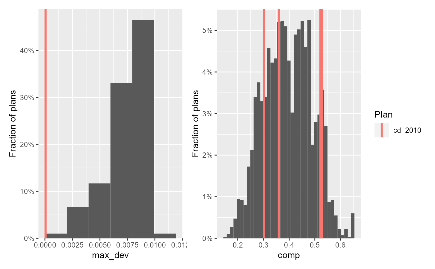
We can see that the adopted plan has nearly complete population parity, and that its districts are roughly as compact on average as those simulated by the SMC algorithm.
One of the most common, and useful, plots, for studying the partisan characteristics of a plan, is to plot the fraction of a group (or party) within each district, and compare to the reference plan. Generally, we would first sort the districts by this quantity first, to make the numbers line up, but here we’ve already renumbered the districts to match the reference plan as closely as possible.
plot(iowa_plans, pct_dem, sort=FALSE, size=0.5)
#> Ignoring unknown labels:
#> • shape : "Plan"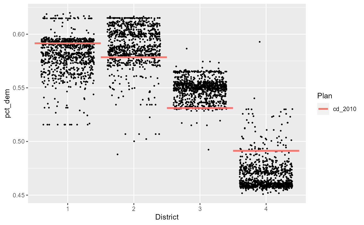
We see that districts 1 and 2 look normal, but it appears that, relative to our ensemble, district 4 (NW Iowa) is more Democratic, and district 3 (SW Iowa, Des Moines) is less Democratic. However, the reference plan does not appear to be a complete outlier.
We might also want to look at how the Democratic fraction in each
district compares to the fraction of minority voters. We can make a
scatterplot of districts, and overlay the reference districts, using
redist.plot.scatter. We’ll also color by the district
number (higher numbers are in lighter colors).
Once again, we see that while district 1 and 2 of the reference plan look normal, district has a lower number of Democrats and minority voters than would otherwise be expected.
pal = scales::viridis_pal()(5)[-1]
redist.plot.scatter(iowa_plans, pct_min, pct_dem,
                    color=pal[subset_sampled(iowa_plans)$district]) +
    scale_color_manual(values="black")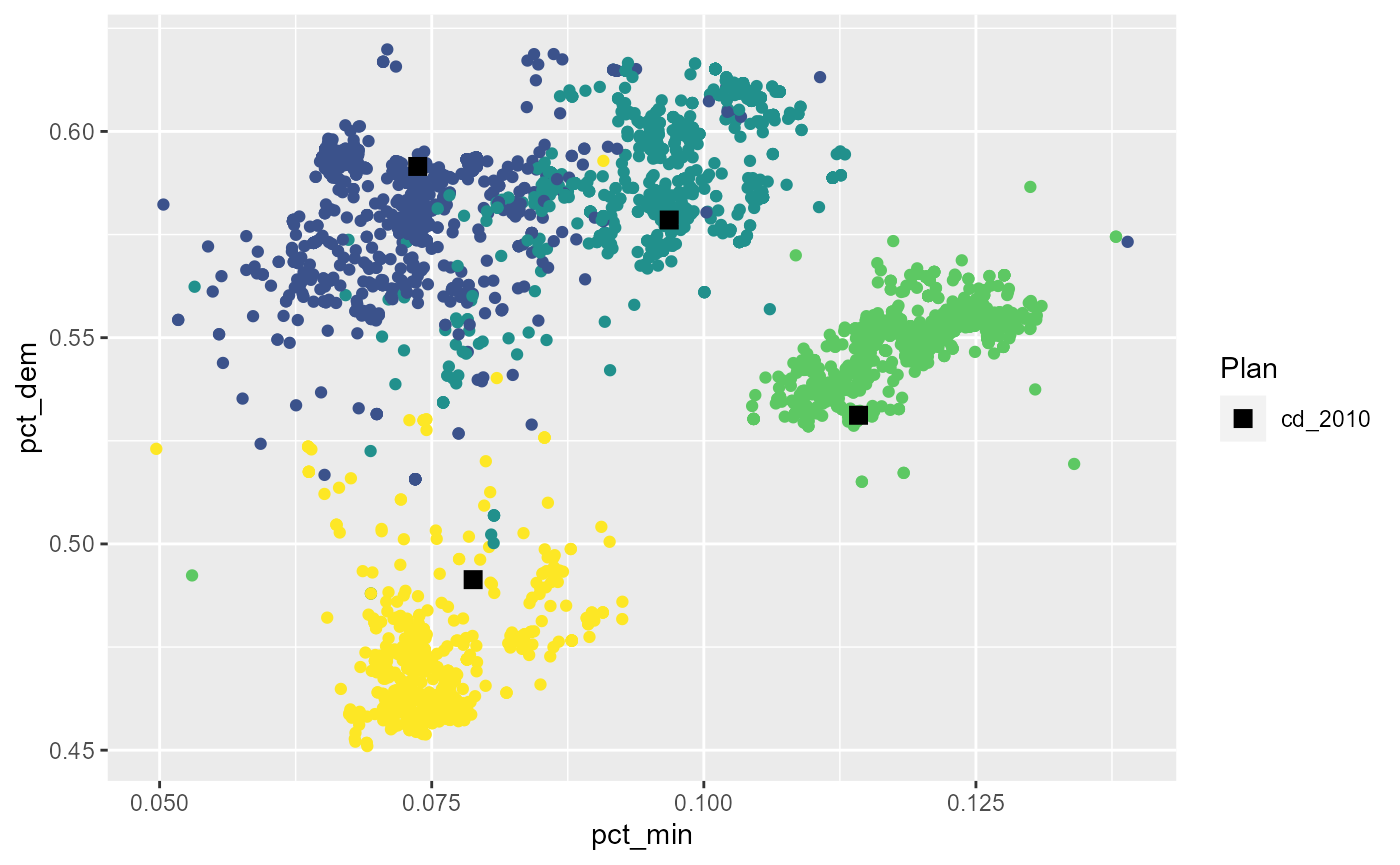
From here, it is easy to keep exploring, using the functionality of
redist_plans and the built-in plotting functions. More
complex model-based analyses could also be performed using the
district-level or plan-level statistics.
